


HMMs, or hidden Markov models, provide a formal framework for developing probabilistic models of 'labelling' issues using linear sequences 1,2. They provide a set of conceptual tools for making complicated models via intuitive picture-drawing. Gene discovery, profile searching, multiple sequence matching, and identifying regulatory sites all rely on them heavily. When it comes to computational sequence analysis, HMMs are like Legos.
A machine learning course can be helpful to get a better understanding of this subject.
As an example, consider the following:
Parameters of a hidden Markov model's probability distribution (example) for better learning:
the X - nation states
potential observations y
chances of changing states
b — Possibilities of Results
A hidden Markov process, in its discrete version, may be thought of as an extension of the urn problem with replacement (where each item from the urn is returned to the original urn before the next step).
Let's say a genie is hiding in a chamber that no one can see. There are urns labelled X1, X2, X3,... throughout the room, and within each urn is a collection of balls with the labels y1, y2, y3,... The genie picks an urn at random and selects a ball from among the balls within. The ball is then placed on a conveyor belt, from which the viewer may see the balls in order but not the urns from whence they were pulled. The genie employs some method to choose urns, with the selection of the urn for ball n depending only on a random number and the selection of the urn for ball (n 1). Thus, this is an example of a Markov process, as the next urn selected does not rely on the selections that came before it.
This configuration is known as a "hidden Markov process" since it is impossible to witness the Markov process directly but only the sequence of labelled balls. As seen in the bottom section of Figure 1, balls y1, y2, y3, and y4 may be drawn in each possible condition. Even if an observer knows the composition of the urns and has just watched a series of three balls, such as y1, y2, and y3, on the conveyor belt, he cannot be certain of the accuracy of this. An observer, however, may deduce additional details, such as the probability that the third ball originated from each of the urns.
Weather guessing game:
Consider long-distance friends Alice and Bob, who have regular phone conversations about their lives. Walking in the park, going to the mall, and tidying up his flat are the only things that fascinate Bob. As so, the day's weather is the only factor in deciding what to do. In terms of specific weather details, Alice is completely clueless, although she is aware of patterns. Alice attempts to infer the weather from Bob's daily descriptions of his activities.
A Markov chain is how Alice imagines the weather to work in discrete increments. The two conditions, "Rainy" and "Sunny," exist but are opaque to her direct perception. Depending on the temperature and humidity, Bob may go for a stroll, go shopping, or clean the house on any given day. As Bob updates Alice on his day, they are the facts that may be gleaned. Each component is a secret Markov model, making up the overall system (HMM).
A data science and machine learning course can be helpful for you to get a better insight into this topic.
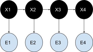
Structural architecture:
Below is a schematic depicting the overarching structure of an HMM implementation. One possible value for a random variable is represented by each oval. Since the hidden state at any given moment t is a random variable, x(t) (using the model shown in the preceding picture, x(t) x1, x2, x3 ). The observation at time t is represented by the random variable y(t) (where y(t) y1, y2, y3, y4 ). Sometimes dubbed a "trellis diagram," the arrows in this graphic depict causal relationships between variables.
It is evident that the value of the hidden variable x(t 1) is the only factor that affects the conditional probability distribution of x(t) at time t, given the values of the hidden variable x at all times. The Markov property describes this phenomenon. Like x(t), the value of y(t) is independent of all other factors except time (both at time t).
The discrete state space of the hidden variables in the usual hidden Markov model addressed here allows for both discrete (generally produced from a categorical distribution) and continuous observations (typically from a Gaussian distribution). Two kinds of parameters may be adjusted in a hidden Markov model: transition probabilities and emission probabilities (also known as output probabilities). Given the hidden state at time t, the transition probabilities determine the hidden state at time t.
t-1.
To simplify the modelling, we suppose that the hidden state space may take on one of N possible values. (For other options, please refer to the "Extensions" section.) That is to say, there is a transition probability from every given state of a hidden variable at time t to any given state of the hidden variable at time t+1, where N is the number of potential states of the hidden variable.
Statistics of N2 transitions. You should know that the total of the probability of all transitions from any state must equal 1. And thus the N\times A Markov matrix is a Nby Nmatrix of transition probability. Given the probabilities of all previous transitions, it is possible to calculate the likelihood of any given transition.
A transition with N(N-1) parameters.
A machine learning online course can enhance your skills.


