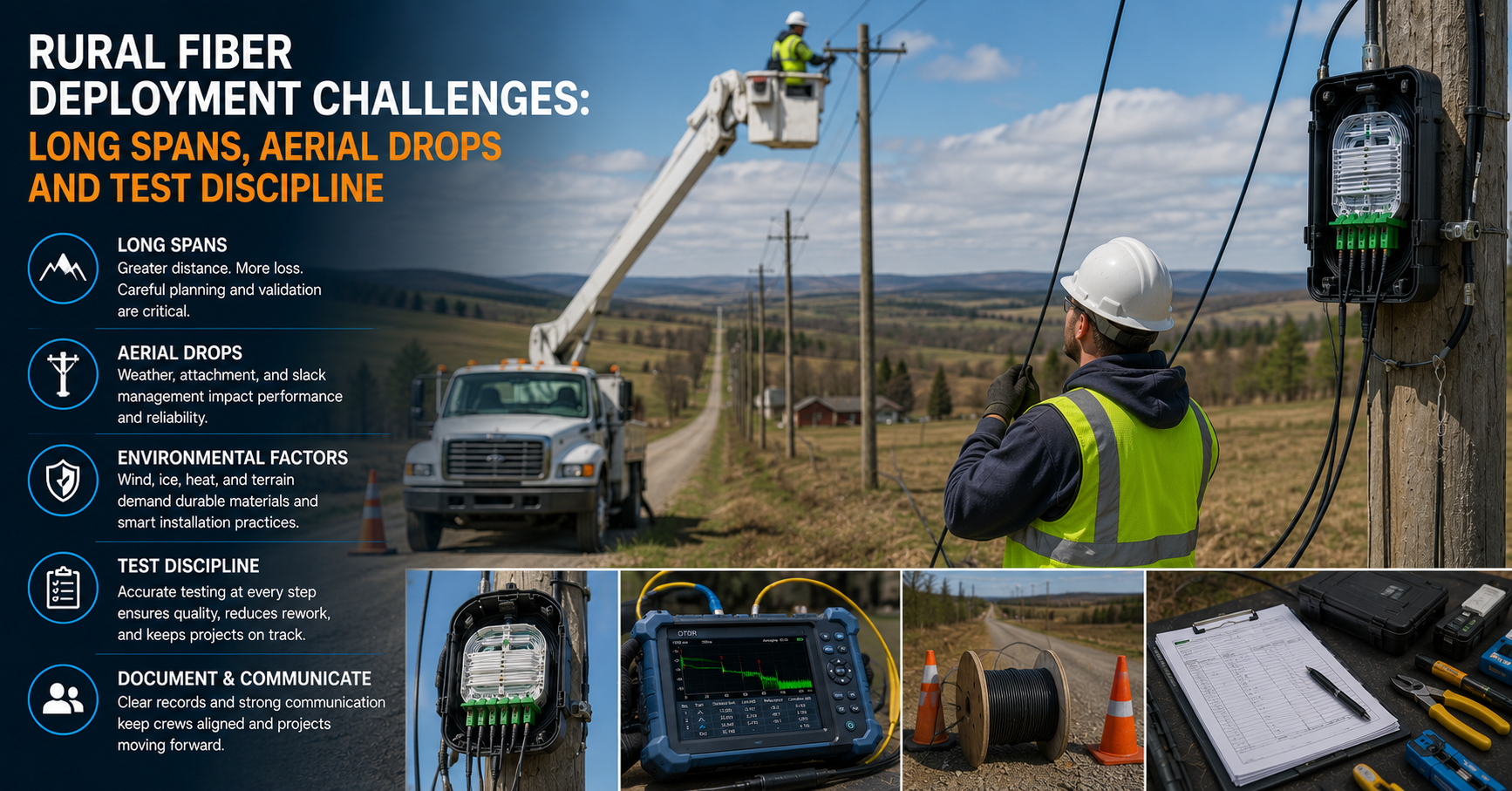
Rural fiber deployment challenges are the engineering, permitting and quality-control problems that appear when a network has to cross long distances to reach very few subscribers, which forces longer pole spans, more exposed aerial drops, thinner access to power and roads, and far higher costs for every defect found after handover. In dense urban builds, a bad splice is a truck roll across town. In a county where the nearest crew is ninety minutes away on a gravel road, the same splice is a full day and a fuel bill.
That distance changes the economics of every decision, and it is why rural fiber optic installation programs live or die on test discipline rather than construction speed.
What Rural Fiber Deployment Challenges Actually Look Like
The word "rural" hides a very specific cost structure. A route that passes 400 homes per mile in a suburb might pass four per mile in farmland, so the same strand of cable has to be paid for by a hundredth of the customers. Every additional pole, every extra splice case and every re-test lands on a much smaller revenue base.
Federal funding has changed the volume of rural broadband fiber deployment work without changing the physics of it. The Broadband Equity, Access, and Deployment (BEAD) Program is a $42.45 billion federal grant program funded by the IIJA, with allocation amounts announced for all 56 states and territories in June 2023. NTIA stated in December 2024 that it had obligated all $42.45 billion in BEAD funding to states. Per NTIA's BEAD Progress Dashboard, all 56 states and territories have submitted their Final Proposals, 55 have received NTIA approval, and NIST has approved 54 of those, making the grant funds available. The bottleneck has moved from paperwork to poles, crews and acceptance testing.
Why Rural Routes Behave Differently From Urban Ones
Density Math and Cost per Passing
Urban builds recover cost through take rate; rural builds recover it through longevity. A rural distribution run may remain in service for decades, which makes installation quality important long after construction ends. Designers who treat rural plant as "urban plant, stretched" end up rebuilding it.
The funding model reinforces this. Most BEAD awards require a 25 percent non-federal match, and all projects must comply with Build America, Buy America sourcing requirements through at least 2029. Rework is not just an operational cost in that model, it is a margin event.
Terrain, Access and Weather Windows
Rural routes cross drainage ditches, rail lines, river banks and private easements that each carry their own permit clock. Frozen ground, harvest season and fire restrictions can close a construction window for months. Crews compress work into short seasons, and compressed schedules are when inspection steps get skipped.
Access shapes the repair plan, not just the build plan. A closure placed at the bottom of a slope for construction convenience becomes unreachable when that slope is saturated. Good rural design puts closures where a bucket truck can still park in March.
Long Spans: Sag, Tension and Fiber Strain
Long-span aerial fiber is the most distinctive feature of rural aerial fiber deployment. Pole lines follow section roads and property boundaries rather than block grids, so distances between support points stretch well past what standard cable is rated for. Span length drives sag, sag drives tension, and tension drives strain on the glass itself.
The governing principle belongs at the front of any span discussion: the sag-tension calculation for the specific route always overrides a catalogue figure. Allowable span depends on rated tensile strength, permitted installation and long-term tensions, span geometry, wind and ice loading, temperature range, attachment hardware and pole condition, read against the manufacturer's design tables. Cable construction narrows the candidate list; it does not by itself set the span.
Fiber strain limits are equally specific to the product. Excessive tension under ice or wind loading can induce micro-bending and macro-bending, which raises attenuation, so allowable strain should come from the cable's published mechanical parameters rather than a rule of thumb. Temporary installation strain and long-term installed strain are usually specified separately, and both need to be respected.
Choosing Between ADSS, Figure-8 and OPGW
Cable construction indicates a working range rather than a hard limit. Central-tube ADSS designs are commonly applied to shorter spans, while layered-twist (stranded) designs are typically offered for longer spans with fiber counts from 48 to 144. Higher-strength designs with RTS values in the 30 to 50 kN range are marketed for spans of several hundred metres and beyond. Commercial ADSS catalogues cover a broad set of span configurations, so the design table for the specific product governs.
Cable geometry feeds back into loading. A typical 24-fiber figure-8 cable measures around 9.5 x 17.2 mm including the messenger, while a 24-fiber ADSS is nearer 11 to 13 mm and a 144-fiber ADSS runs 15 to 18 mm. Larger diameter means more surface for wind and ice to act on, which is why over-specifying fiber count on a long span can quietly force a stronger and more expensive cable.
Practical selection notes:
- ADSS: all-dielectric and self-supporting, carrying load through aramid strength members with no metallic elements, which suits joint-use structures.
- Figure-8: incorporates an integrated messenger, which can be metallic or dielectric depending on the cable design, and is common on straightforward telecom-only pole lines.
- OPGW: used on transmission structures where the cable also serves as shield wire.
- Jacket selection: track-resistant jackets are specified where the cable runs in the induced-field region of higher-voltage conductors.
NESC Loading Districts and Clearance Rules
Where the NESC applies, its clearance rules establish minimum requirements that designers and utilities must account for, alongside the applicable code edition, utility construction standards and jurisdictional requirements. NESC Table 232-1 sets minimum vertical distances, commonly cited as 15.5 feet over roads and streets subject to truck traffic, 15 feet over driveways and parking areas not normally used by heavy vehicles, and 9.5 feet over spaces limited to pedestrians only. The reduced pedestrian figure is one of the most frequently misapplied rules, because the NESC defines a roadway to include its shoulder.
Vertical separation on the pole is governed by its own rules and configurations. The NESC defines a communication worker safety zone, cited in reference material as 40 inches of clearance between communication lines and supply lines or equipment under Rules 235C4 and 238E, and the clearance that actually applies depends on the arrangement and the rules invoked for it. Ice and wind loading is applied by district, and northern utilities may impose requirements more stringent than the NESC baseline where icing is frequent and severe.
Pole Attachment and Make-Ready Realities
Make-ready is where rural schedules usually slip, and it is one of the most underestimated rural fiber deployment challenges in project planning. Pole owners must survey, engineer and often physically rearrange existing attachments before a new communications cable can be hung, and in rural areas the pole population is older, more mixed in ownership and less well documented. A single non-compliant pole can hold up an entire span sequence.
The sequence itself is the lever. Field surveys should capture pole class, existing attachment heights, guying and ground clearance in a single visit, because a second trip to a remote line is disproportionately expensive. Crews that photograph every pole face during the walk-out cut their engineering rounds sharply.
Aerial Drops: The Exposed Edge of Last Mile Fiber Deployment
Drop Cable Selection and Bend Radius
Fiber optic drop cable installation is where rural FTTH deployment meets weather, wildlife and homeowners. Drops run from a distribution point to a farmhouse across an open yard, often with no intermediate support and no shelter from wind. Bend-insensitive fiber to ITU-T G.657.A1 or G.657.A2 tolerates the tight radii that appear at the NID far better than standard G.652.D.
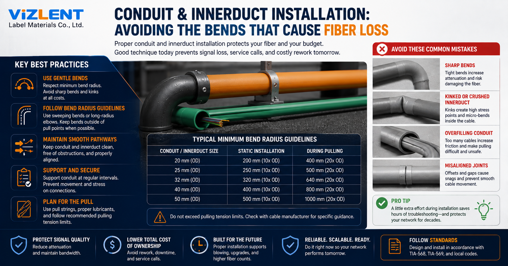
Installation habits matter more than cable grade. Over-tightening a dead-end clamp, stapling a drop to a fascia board or coiling slack too tightly all create bend loss that will not show on a simple continuity check. A slack loop sized to the manufacturer's minimum bend radius costs nothing and prevents a return visit.
Storm Damage and Repair Access
Aerial drops fail in patterns, and rural patterns are predictable: falling limbs, ice accretion, vehicle strikes at driveway crossings and rodent damage at the pole. Designing for the site's applicable wind and ice loading conditions is cheaper than repeatedly repairing storm damage. That means using the loading district and any utility-specific overlay that governs the route, not a generic assumption.
Restoration speed depends on records, which is where rural fiber maintenance is won or lost. Legible fiber assignments in the closure, drop lengths recorded at install and OTDR baselines on file turn a four-hour fault hunt into a forty-minute fix. Networks without those records rediscover their own topology during every outage, in the dark.
Contamination: The Failure Mode Nobody Budgets For
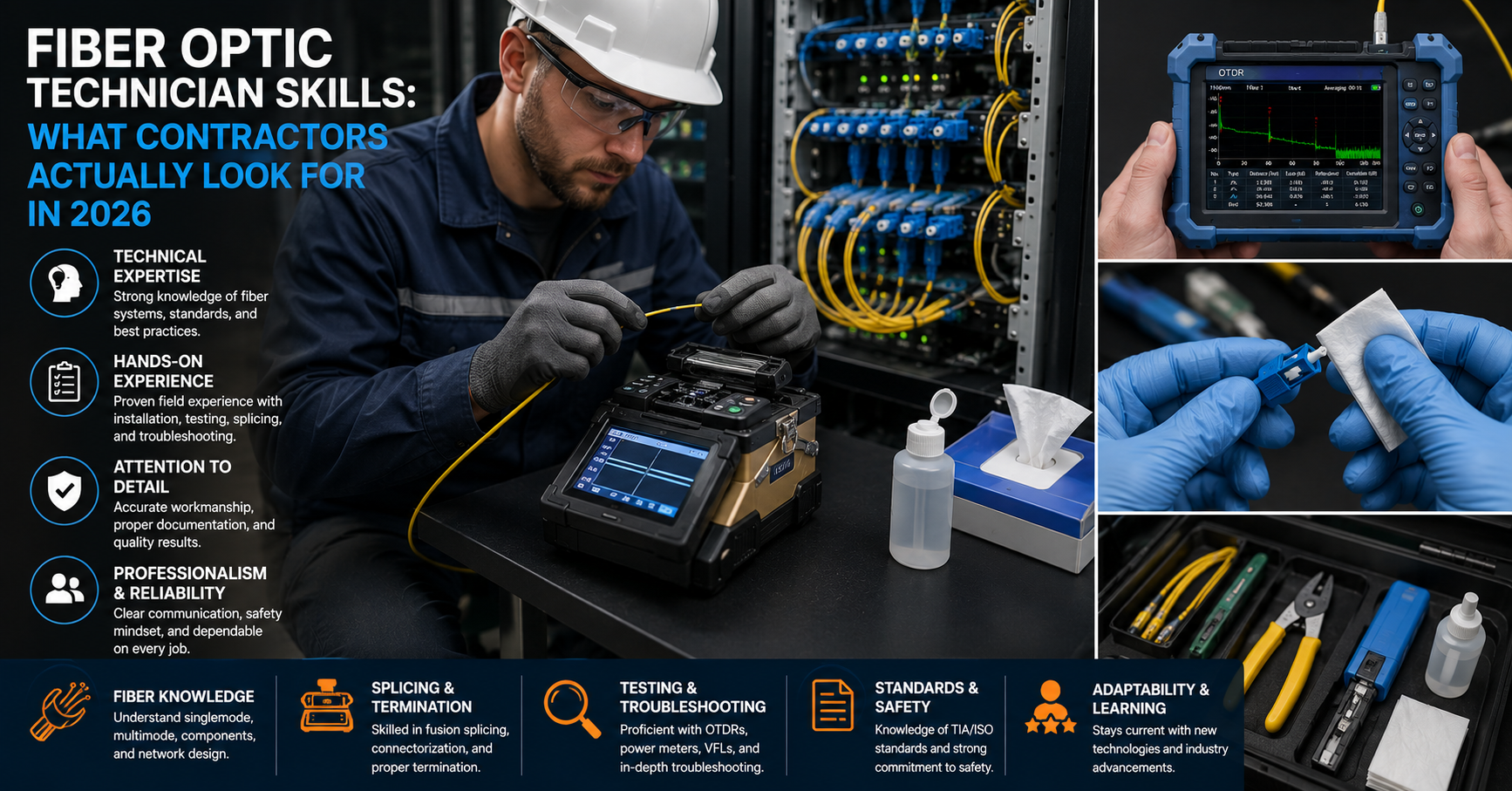
End-face contamination is a common and preventable cause of rural fiber acceptance failures. A particle a few microns across is invisible on the bench yet enough to scatter light, raise insertion loss and damage the glass when two ferrules mate under optical power. Dust, splice-gel residue and fingerprints arrive free with every field connection.
Method has to match the contaminant. Dry mechanical cleaning with purpose-built fiber cleaning tools lifts particulate without leaving residue, while oils and gels need a wet-then-dry pass so the film is dissolved and carried off before it dries into streaks. Improvised cloths and improperly applied alcohol can leave residue, generate lint or redistribute contamination across the end face, which is why lint-free media and optical-grade solvent are specified rather than assumed.
The acceptance criteria are published, not subjective. IEC 61300-3-35:2022 specifies the procedure and pass/fail criteria for inspecting fibre-optic end faces for cleanliness, covering zones A and B on the fibre plus the whole contact area, up to 250 µm diameter for cylindrical ferrules. Inspect and clean connector end faces before mating and testing, following the applicable inspection procedure for the connector type in use.
A workable field loop looks like this:
- Inspect the end face with a scope before every mate.
- Clean dry first if the failure is particulate.
- Clean wet-then-dry only if a film or residue is present.
- Re-inspect, and repeat only on the zone that failed.
- Cap the connector immediately if it is not being mated.
Test Discipline: Tier 1, Tier 2 and Bidirectional Traces
Setting a Realistic Loss Budget
Loss budgets are where optimistic design meets measured reality, and rural routes expose the gap fastest. A defensible budget starts from the ITU-T G.652.D attenuation specifications of 0.4 dB/km at 1310 nm and 0.3 dB/km at 1550 nm, then adds allowances for each fusion splice, each connector pair and any splitters in a PON design. Those figures are maximum fiber attenuation specifications rather than the actual attenuation of the deployed cable or the complete link-loss budget, and deployed cable frequently performs better.
The reference method affects the number reported. TIA and ISO/IEC cabling standards define 1-jumper, 2-jumper and 3-jumper methods, with the 1-jumper method preferred in the TIA standard and the 3-jumper method preferred in ISO. The current editions are ANSI/TIA-568.3-E and ISO/IEC 14763-3:2024, so test plans written against older editions should be checked before they are reused. Two crews using different reference methods on the same link will produce different results, and neither is wrong.
OTDR Setup for Long Rural Spans
Tier 1 and Tier 2 are not interchangeable. Tier 1 certification uses an optical loss test set to measure insertion loss, length and polarity, and it is the baseline defined in the TIA field-testing guidance. Tier 2 adds an OTDR to characterise each event along the link. Tier 2 is listed as optional in the TIA standard, but the trace supports cable acceptance, splice and connector loss, documentation, fault location and optical return loss. An OTDR trace does not replace Tier 1 insertion-loss testing when certification requires the TIA Tier 1 baseline.
Setup choices decide whether the trace is usable. OTDR traces should be acquired at the same wavelengths used for Tier 1. Bidirectional OTDR analysis improves event-loss accuracy, particularly for splice and connector characterisation, because it reduces directional measurement effects that single-ended acquisitions cannot resolve. Many network owners and project specifications require Tier 2 OTDR documentation because it provides event-level information that Tier 1 cannot.
For rural OTDR testing, a few setup rules do most of the work:
Use a launch fiber long enough to move the near-end connector out of the event dead zone, and a receive fiber to characterise the far-end connector.
- Match pulse width to span length: short pulses for resolution near the OLT, longer pulses to reach the far end of a long feeder run.
- Test at 1310 nm and 1550 nm, and use 1625 nm or 1650 nm where the network design, maintenance procedure and test equipment support it, particularly for in-service troubleshooting with appropriate filtering.
- Set the refractive index from the cable datasheet, not from the instrument default, or distances will be wrong.
- Save the trace file, not just the pass/fail summary.
Kit specification follows from that list rather than the other way round. Where a route includes long feeders and multiple splice points, dynamic range and event dead zone are the two specifications that decide whether a trace is diagnostic or merely reassuring, which is the practical case for selecting an OTDR tester on span length rather than on price.
Documentation, Handover and Grant Compliance
Grant-funded rural broadband infrastructure carries an evidentiary burden that private builds often do not. Subgrantees are typically asked to show that each location was actually served and that the plant meets the performance the award was scored on, which turns test records into compliance artefacts. Losing a trace file is not a technical problem in that context, it is an audit problem.
Structure the record set at design time rather than at closeout. One folder per route, holding the as-built, the splice matrix, Tier 1 results, Tier 2 traces and end-face inspection reports, satisfies most reviewers. Retrofitting that structure after 300 miles of construction is where projects lose weeks.
Why Rural Fiber Requires More Upfront Discipline
Discussions of rural fiber deployment challenges and benefits usually stop at cost per passing, which understates what disciplined construction actually buys. Rural plants are expensive to reach, so the return on getting it right the first time is proportionally larger than in a dense build. The upfront work is design, inspection and documentation; the return is measured over the asset's service life.
Where that discipline pays back:
- Longer asset life: clean, correctly tensioned plant is not carrying latent mechanical or optical defects into its second decade.
- Fewer truck rolls: faults that were never installed do not need to be driven to.
- Faster fault localisation: an archived OTDR baseline turns a search into a comparison, and as-builts assembled during construction survive staff turnover.
- Lower lifecycle cost: capacity headroom on a rural fiber optic network means upgrades are electronics swaps rather than rebuilds.
Rural Fiber Deployment Challenges at Work: A Field Checklist
Seeing rural fiber deployment challenges at work usually means watching a crew make a small decision under time pressure. The checklist below is deliberately short, because long checklists get ignored at 4 p.m. in the rain.
Before the crew leaves the site:
- Sag measured and compared against the design table for the cable and loading district.
- Ground clearance verified at mid-span, not at the pole.
- Every mated connector inspected against IEC 61300-3-35 criteria, which is where field-grade fiber optic inspection scopes earn their place in the kit.
- Splice losses recorded per fusion, bidirectionally where the specification calls for it.
- Drop slack coiled at or above the minimum bend radius.
- Trace files named by fiber ID and stored, not left on the instrument.
Two habits separate crews that come back from crews that do not. The first is inspecting before mating rather than after failing. The second is writing the number down at the pole, because reconstructed data is the same as no data.
Frequently Asked Questions
What causes most rural fiber deployment challenges during construction?
Most problems trace back to span length and access rather than to the fiber itself. Longer spans raise sag and tension, which raises the risk of exceeding the cable's specified mechanical limits, while limited road access makes every correction expensive. Permitting and make-ready delays then compress the schedule, which is when inspection and cleaning steps get skipped.
How long can an aerial fiber span be in a rural build?
Span length is set by the sag-tension calculation for the specific route and cable, not by a single catalogue number. Allowable span depends on the cable's rated tensile strength, permitted installation and long-term tensions, span geometry, wind and ice loading, temperature range, attachment hardware and pole condition. Cable construction narrows the candidate products, and the manufacturer's design tables determine what the route will support. Ice and wind loading typically reduce achievable span substantially against fair-weather figures.
Is Tier 2 OTDR testing required on rural fiber networks?
Tier 2 is listed as optional in the TIA field-testing guidance, while Tier 1 loss testing with an optical loss test set is the baseline. Many network owners and project specifications nevertheless require Tier 2 documentation, because the OTDR trace locates events along the link in a way Tier 1 cannot. That matters most when the next technician is hours away.
Why does end-face cleaning matter more on rural routes?
The consequence of a dirty connector scales with how hard it is to get back to it. Contamination raises insertion loss and reflectance, and a contaminated end face can be physically damaged the moment it mates under optical power. Because rural sites are dusty and drops are handled outdoors, contamination rates run higher than in a controlled environment, making inspection before every mate the cheapest quality step available.
What is the difference between ADSS and figure-8 cable for rural spans?
ADSS is all-dielectric and self-supporting, carrying its own load through aramid strength members with no metallic elements. Figure-8 cable incorporates an integrated messenger, which can be metallic or dielectric depending on the cable design, and the choice affects where the cable can be placed relative to energised conductors and whether bonding and grounding are required. ADSS is generally preferred on joint-use or utility structures, while figure-8 remains common on telecom-only pole lines.
How do NESC clearance requirements affect rural design?
Where the NESC applies, Table 232-1 sets minimum vertical clearances the cable must maintain at final sag, including the commonly cited 15.5 feet over roads subject to truck traffic. Because sag increases with span length, temperature and ice loading, the governing case is rarely the day of installation. Separation on the pole is governed by its own rules and configurations, and field verification should be taken at mid-span rather than at the attachment point.
What loss budget should a rural PON link be designed to?
The budget is built from the fibre attenuation, the connector pairs, the fusion splices and any optical splitters in the path, then checked against the class of optics deployed. ITU-T G.652.D specifies maximum attenuation of 0.4 dB/km at 1310 nm and 0.3 dB/km at 1550 nm, and these are specification limits rather than the attenuation the deployed cable will actually show. Long feeder runs make the fibre term a large contributor, and splitter loss is fixed by ratio.
Which records should be handed over at project closeout?
At minimum, the as-built route drawing, the splice matrix, Tier 1 loss results, Tier 2 OTDR trace files and end-face inspection reports for every mated connector. Grant-funded projects frequently need this evidence tied to specific serviceable locations rather than to route segments. Storing raw trace files rather than pass/fail summaries preserves the ability to re-analyse later, and records assembled during construction are consistently more complete than records assembled at closeout.
Where to Focus Next
Rural fiber deployment challenges reward preparation far more than speed, and the payoff sits in three places: a sag-tension design that respects the cable's published parameters and the loading district, an inspect-and-clean loop that runs before every mate, and a bidirectional test record that survives the project. Crews that hold those three lines produce a plant that stays quiet for a decade.
If a rural build is in planning, audit what each crew actually carries against the route it will work: connector types present, longest feeder to be tested, and whether inspection and cleaning consumables are sized for both. That audit usually surfaces more avoidable loss than any change to cable specification.