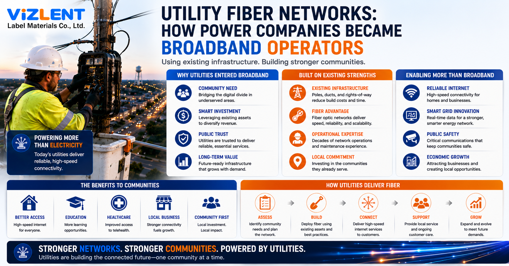
Utility Fiber Networks: How Power Companies Became Broadband Operators

Utility fiber networks are optical cable systems built and owned by electric utilities, originally to carry protection and control traffic between substations, and later extended to deliver commercial broadband to homes and businesses along the same poles and ducts. The shift happened because the hard costs of fiber deployment, the poles, the rights-of-way, the trucks, the line crews, were already paid for by the electricity business. Once a utility strings a cable to every substation, the marginal cost of adding fibers for retail service is small compared to what a greenfield ISP would spend.

That economic accident has turned power companies into some of the most capable broadband operators in rural America. It has also handed their engineering teams a discipline most electrical engineers never trained for: optical link design, where a single fiber optic loss budget determines whether a 40 km feeder route can carry service at all. The engineering, the economics, and the regulatory friction all trace back to that one calculation.

Why Electric Utilities Own So Much Fiber

Electric utilities began installing optical fiber in the 1980s for reasons that had nothing to do with the internet. Protective relaying between substations needs deterministic, low-latency communication that is immune to the enormous electromagnetic fields around high-voltage conductors, and glass is immune by construction. Copper pilot wires could not survive the induced voltages, so fiber became the default medium for teleprotection, SCADA, and later synchrophasor measurement.

The second driver was grid automation. Utilities that wanted self-healing distribution circuits needed a communications path to every reclosing switch, capacitor bank, and smart meter concentrator on the feeder. Chattanooga's EPB is the clearest example: its fiber plant connects more than 1,400 automated switches that reroute power around faults, and the utility credits that architecture with roughly halving annual outage minutes.

Typical utility applications riding the same glass include:

• Line differential and distance protection between substations
• SCADA and distribution automation telemetry
• Advanced metering infrastructure backhaul
• Substation video, physical security, and environmental monitoring
• Corporate WAN traffic between service centers and control rooms

How Fiber Utility Networks Became Retail Broadband

Once the backbone existed, the spare fiber count became an asset looking for a use. Utilities routinely install 48, 96, or 288-fiber cable when only a handful of strands serve grid functions, because the cost of the cable is trivial next to the cost of hanging it. Selling or leasing the surplus was the first commercial step, and dark fiber leasing to carriers and wireless operators still funds a large share of utility telecom divisions.

Retail service came next, mostly in places incumbent carriers refused to build. According to the National Rural Electric Cooperative Association, more than 250 electric co-ops are now deploying or planning broadband for their members. Municipal utilities followed a parallel path, and the growth of electric cooperative broadband has made utilities the fastest-expanding category of fiber-to-the-home providers in low-density markets.

The commercial models generally fall into four buckets:

• Dark fiber leasing. The utility sells strands and lets the tenant light them.
• Middle-mile transport. The utility lights the network and sells wavelengths or Ethernet circuits to ISPs and carriers.
• Open access. The utility owns the optical distribution network and multiple retail ISPs compete over it.
• Vertically integrated retail. The utility operates its own ISP subsidiary and bills the end subscriber directly.

The Cable Types That Define Utility Fiber Optic Plant

Utility fiber optic construction uses cable designs that telecom engineers rarely encounter. Optical ground wire, or OPGW, replaces the shield wire at the top of a transmission structure and performs two jobs at once: it intercepts lightning and grounds fault current while carrying fibers inside an aluminum-clad steel tube. Its construction and testing are governed by IEEE 1138, which covers short-circuit current capacity, sag and tension, and the fiber's optical performance under mechanical strain.

All-dielectric self-supporting cable, or ADSS, contains no metal at all, which is why it can be installed on energized distribution lines without a bonded path to ground. IEEE 1222 governs its performance, and placement decisions hinge on the space potential at the attachment point, because dry-band arcing will erode a jacket that sits in too strong an electric field. Underground routes use conventional loose-tube or ribbon cable in duct, often shared with the utility's own conduit system.

Practical differences that matter to design:

• OPGW spans are long, often 300 metres or more, with splice points restricted to structures where crews can safely work
• ADSS is lighter and cheaper to install but sensitive to electrical field strength and track-resistant jacket selection
• Both designs concentrate splices at towers and poles rather than at convenient handholes, which drives up splice counts more than most planners expect

Why the Fiber Optic Loss Budget Governs the Business Case

A fiber optic loss budget is the calculated total optical power, expressed in decibels, that a link can lose between transmitter and receiver while still meeting its bit error rate target. It is the arithmetic that decides how far a utility can reach from a substation, how many subscribers can hang off one splitter, and whether an expensive intermediate site is required. Get it wrong on paper and the cost shows up later as an unplanned regeneration hut or a rebuilt splice point.

For utility broadband, the number is not academic. A GPON system built to the ITU-T Class B+ specification supports a maximum optical path loss of 28 dB, with C+ optics reaching 32 dB, while XGS-PON defines N1 and N2 classes at 29 dB and 31 dB. Every metre of cable, every splitter, and every connector spends part of that allowance, and the fiber optic loss budget is simply the ledger that tracks the spending.

Building a Fiber Optic Loss Budget Line by Line

The calculation itself is straightforward addition, and the discipline lies in refusing to be optimistic. Standard single-mode fiber to ITU-T G.652.D specifies attenuation no greater than 0.4 dB/km at 1310 nm and 0.3 dB/km at 1550 nm, though production fiber usually performs better. Fusion splices are typically budgeted at 0.1 to 0.3 dB each, and ANSI/TIA-568.3 allows a maximum of 0.75 dB per mated connector pair.

A worked example makes the pressure visible. Consider a 22 km feeder from a substation to a rural cabinet, with 12 splices, four connector pairs, and a 1:32 splitter rated at 17.5 dB insertion loss. The fiber optic loss budget adds up like this:

• Fiber attenuation: 22 km x 0.35 dB/km = 7.7 dB
• Fusion splices: 12 x 0.15 dB = 1.8 dB
• Connectors: 4 x 0.5 dB = 2.0 dB
• Splitter: 17.5 dB
• Subtotal: 29.0 dB

Against a Class B+ budget of 28 dB, that link fails before a single subscriber is connected. Against C+ optics at 32 dB it passes, but with only 3 dB of headroom, which is roughly what a prudent engineer reserves for aging, temperature drift, and future repair splices. Utilities in this position usually drop to a 1:16 splitter, move the splitter closer to the customer, or accept XGS-PON N2 optics.

Where Utility Routes Quietly Burn Margin

Utility corridors punish loss budgets in ways that suburban telecom routes do not. Transmission rights-of-way rarely run in a straight line toward customers, so route kilometres often exceed map kilometres by 30 percent or more, and every extra kilometre is spent from the same fiber optic loss budget. Splice-point placement is dictated by structure access rather than optical convenience, which adds counts that no desktop model predicted.

Contamination is the second silent tax. Utility crews terminate in substations, cabinets, and hand holes where dust, insects, and hydraulic mist are ordinary, and a contaminated end face can add loss and reflectance far beyond specification. Disciplined use of fiber cleaning tools before every mating, verified against the IEC 61300-3-35 end-face grading criteria, is the cheapest protection a utility fiber optic program can buy.

Common margin thieves worth auditing on any utility build:

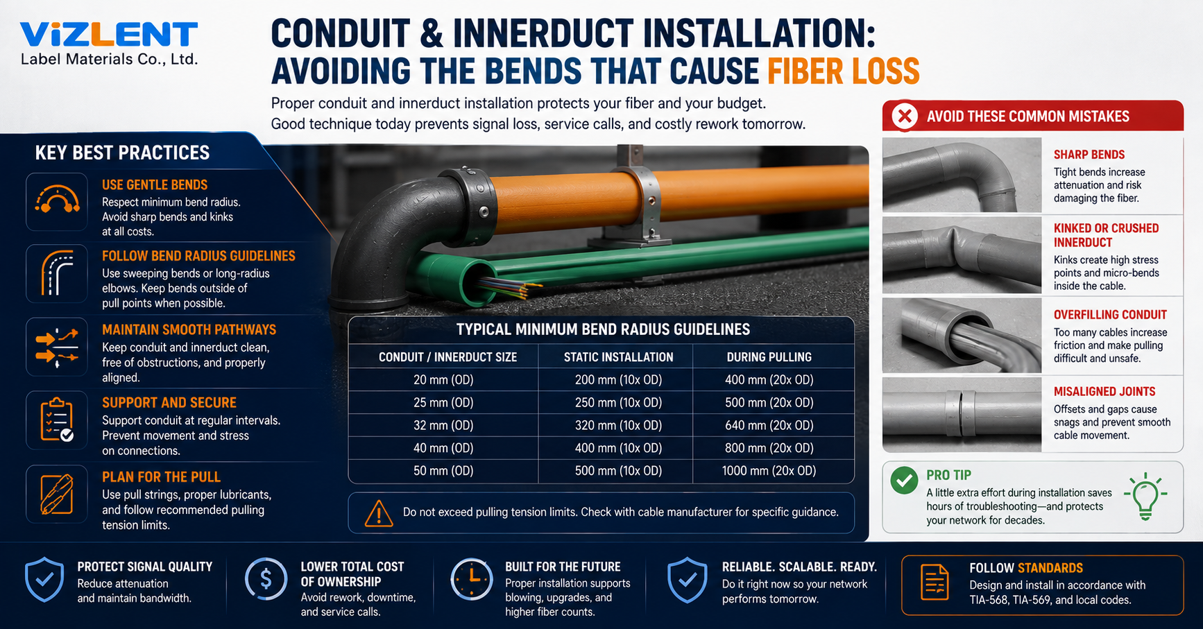
• Macrobends at storage loops on tower legs and in undersized enclosures
• Extra splices added during storm restoration and never recorded in the as-built
• Connector reflectance in patch panels that were never inspected after installation
• Wavelength drift, since a link engineered at 1310 nm behaves differently at 1550 nm
• Splitter ratios chosen for take-rate optimism rather than measured loss

Planning a utility route? Build the loss budget before the route survey, not after. The design decisions that follow, splitter placement, cable count, and optics class, are all downstream of that number.

Testing and Commissioning Utility Fiber Services

Commissioning a utility fiber network follows the same two-tier logic used across structured cabling, and both tiers matter. Tier 1 certification measures end-to-end insertion loss with a light source and an optical power meter, producing the single number that is compared against the design fiber optic loss budget. If measured loss exceeds the calculated allowance, the link is not accepted, regardless of whether traffic appears to pass.

Tier 2 characterisation uses an OTDR tester to map every event along the span, which is what turns a failing number into a located fault. Bidirectional averaging matters on utility routes because splices between fibers of different mode field diameter produce misleading gainers in one direction. The resulting trace becomes the baseline that restoration crews compare against after every storm season.

A defensible acceptance package generally contains:

• The design loss calculation with every assumption stated
• Bidirectional OTDR traces at 1310 nm and 1550 nm
• Tier 1 insertion loss results for every fiber, not a sample
• End-face inspection images for connectors at both ends
• An as-built splice matrix with GPS coordinates for each closure

Regulatory and Easement Realities Behind Utilities & Fibre Networks

Engineering is often easier than the law. Electric easements were typically granted for the delivery of electricity, and using that same corridor to sell retail broadband can fall outside the granted purpose. NRECA has documented cases where co-ops faced significant litigation over exactly this question, and roughly 18 to 20 states have since passed easement relief legislation to resolve it.

Pole attachment economics form the second constraint. A utility that owns its poles avoids the attachment fees and make-ready delays that slow competing ISPs, which is a structural advantage in the utility fiber services market. Utilities entering retail broadband also take on regulatory obligations they never had as a power company, including service quality reporting, customer privacy rules, and in many states a requirement to separate broadband finances from the regulated electric business.

Questions worth settling before construction begins:

• Do existing easements permit commercial telecommunications traffic?
• Does state law authorise the utility or cooperative to offer retail service?
• How will shared costs be allocated between the electric and broadband entities?
• What happens to the fiber asset if the broadband subsidiary is later sold?

What Experienced Utility Teams Do Differently

Utilities that succeed in broadband tend to treat optical plants with the same documentation discipline they apply to protective relaying. Every splice is recorded, every acceptance test is archived, and the fiber optic loss budget is stored as a living document that gets updated when a repair splice is added. That habit sounds bureaucratic until a fault occurs at 2 a.m. and the crew needs to know whether the link had 6 dB of margin or 0.6 dB.

The second habit is conservatism about margin. Experienced designers reserve headroom for at least two future repair splices per span, because storm damage on an overhead plant is a certainty rather than a risk. Teams that spend the whole optical allowance on day one end up rebuilding links after the third restoration, which costs far more than the splitter ratio they were trying to save.

Reviewing an existing utility fiber build? Start by comparing today's measured loss against the original design figures. The gap between them is usually where your reliability problems live.

Building or Auditing a Utility Fiber Network

Fiber utility networks succeed or fail on details that never appear in a business plan: splice counts, end-face cleanliness, and honest margin. If your team is planning a route, calculate the fiber optic loss budget first and let it constrain the design rather than validating it afterwards. If you are inheriting an existing plant, start with measured loss against original design figures and work backwards from the discrepancies.

Whichever position you are in, the tooling matters as much as the mathematics. Reliable inspection, cleaning, and test equipment is what keeps a calculated fiber optic loss budget true in the field, year after year, through every storm restoration and every added splice.

Frequently Asked Questions

What is a fiber optic loss budget?

A fiber optic loss budget is the maximum total optical power a link can lose between transmitter and receiver while still meeting its performance target, measured in decibels. It is calculated by adding fiber attenuation, splice loss, connector loss, and any splitter or component loss along the path. Designers compare that total against the optical budget of the chosen transceivers, then reserve additional margin for repairs and aging.

Why do electric utilities build fiber networks?

Electric utilities build fiber because grid protection, SCADA, and distribution automation require immune, low-latency communications along the same corridors the utility already controls. Fiber is unaffected by the electromagnetic fields surrounding high-voltage equipment, which makes it the only practical medium for substation-to-substation protection signalling. Broadband service is usually a secondary use of capacity installed for those grid functions.

What is the difference between OPGW and ADSS cable?

OPGW is a metallic cable that replaces the overhead shield wire and carries fault current as well as fibers, while ADSS contains no metal and is strung below the conductors on distribution or transmission structures. OPGW suits new transmission construction and lightning-exposed spans, since it performs a grounding function that ADSS cannot. ADSS is generally faster and cheaper to install on existing energised lines because it needs no bonding path.

How many fibers does a utility network actually need for grid operations?

Most grid applications need only a handful of strands per route, often fewer than twelve, since protection and SCADA traffic is low bandwidth by modern standards. Utilities nonetheless install high-count cable because the incremental cost of additional fibers is small compared to the labour of installing the cable. The surplus becomes the basis for dark fiber leasing, middle-mile transport, and last-mile broadband.

Can a utility offer broadband over the same fiber that runs the grid?

Yes, provided the grid traffic is logically or physically separated from commercial traffic. Most utilities dedicate specific fibers or wavelengths to protection and SCADA and keep them isolated from the retail optical distribution network. Regulators and internal security teams typically require documented separation, and some utilities go further by using entirely separate cables for teleprotection.

What loss budget do PON systems use in utility broadband support?

GPON Class B+ optics support up to 28 dB of optical path loss, C+ optics reach 32 dB, and XGS-PON defines N1 and N2 classes at 29 dB and 31 dB respectively. The chosen class determines how far the network can reach and what splitter ratio is affordable. Utilities serving long rural feeders frequently specify higher-class optics precisely because their route lengths consume so much of the available budget.

How often should a utility fiber network be retested?

Baseline acceptance testing happens at commissioning, and most utilities retest a span after any repair splice, storm restoration, or reported performance degradation. Periodic sampling of critical links, commonly annually, catches slow degradation from connector contamination or enclosure water ingress. Comparing new traces against the archived baseline is what makes the retest meaningful.

Are utility fiber networks more reliable than commercial ISP networks?

Utility networks often benefit from redundant ring topologies, in-house line crews, and restoration processes built around storm response, which can translate into faster repair times. Reliability still depends on construction quality, splice discipline, and how much optical margin was reserved at design. A well-documented network with conservative loss budgets outperforms a poorly documented one regardless of who owns it.